
Blog Post 4
In this post, we’re going to implement the spectral clustering algorithm for clustering data points using the numpy and scipy libraries. To begin, we’ll optimize an objective function to output the data classes, but later we’ll use something called a Laplacian matrix which simplifies the clustering process.
Introduction
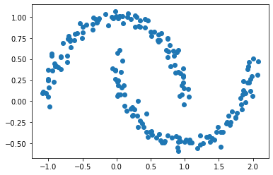
Clustering methods like K-means are used for simple clustering problems—however, when data is shaped “weirdly”, (e.g. two crescent moons next to each other or two cocentric circles), K-means often fails to classify the data (e.g. each of the crescent moons or each of the cocentric circles). Below is an example of the crescent moon data.
np.random.seed(1234)
n = 200
X, y = datasets.make_moons(n_samples=n, shuffle=True, noise=0.05, random_state=None)
plt.scatter(X[:,0], X[:,1])
Spectral clustering is a method that aims to cluster data with complex structure. Below we use optimization to implement the method, before using a shortcut using Laplacian matrices.
Similarity Matrix
We create a similarity matrix A, which is a n x n matrix that uses the Euclidean distance between points X[i] and X[j]. Here, if the distance is less than epsilon (a parameter we can change), entry A[i, j] is 1, but if the distance is more than epsilon, entry A[i, j] is 0.
While the Euclidean distance between the same point is 0 which implies A[i, j] is 1 if epsilon > 0, we make all diagonal entries A[i, i] 0. We create the similarity matrix below.
from sklearn.metrics import pairwise_distances

# set epsilon = 0.4
epsilon = 0.4

# pairwise_distances() with conditional indexing outputs the similarity matrix with 1 for each diagonal entry
A = (pairwise_distances(X) < epsilon).astype(int)

# fill diagonals with 0
np.fill_diagonal(A, 0)
Binary Norm Cut Objective
The next step is to create the binary norm cut objective, which contains the cut and the volume terms. For this, we also use the row-sum, a vector where each element is the sum of the rows of the similarity matrix A. We also use y, the true cluster membership vector, where each element of y (either 0 or 1) indicates what class each point in X lies. The smaller the binary norm cut objective, the better the true cluster membership vector is at differentiating between classes.
The Cut Term
The cut term adds up entries A[i, j], where i indicates each index of the points in the first class and j indicates each index of the points in the second class. We implement a function below that calculates the cut of a matrix given the true cluster membership vector.
def cut(A, y):
    # initialize cut
    cut = 0

    # for each index of y where y[i] == 0
    for i in np.where(y == 0)[0]:

        # for each index of y where y[j] == 1
        for j in np.where(y == 1)[0]:

            # add A[i, j] to cut
            cut = cut + A[i, j]
    return cut

cut(A, y)
13
To show that the cut objective works, we use a vector of random integers to replace y, and compare the cut objective.
np.random.seed(1234)
cut(A, np.random.randint(2, size = n))
1154
The cut objective for a vector of random integers is much larger, meaning a random vector is not good at differentiating classes.
The Volume Term
The volume term for a cluster is the sum of row sums d[i], where i is the index of terms in one cluster in y. We implement a function below that calculates the volume of a matrix given the true cluster membership vector.
def vols(A, y):
    # row sum
    d = np.sum(A, axis = 1)

    # returns a tuple of the sum of row sums for the first cluster and the second cluster
    return (np.sum(d[np.where(y == 0)[0]]), np.sum(d[np.where(y == 1)[0]]))

vols(A, y)
(2299, 2217)
The volume of cluster 0 is 2299 and the volume of cluster 1 is 2217.
The Normcut Objective
We implement a function calculating the normcut objective using the cut() and vols() functions above.
def normcut(A, y):
    return cut(A, y) * ((1 / vols(A, y)[0]) + (1 / vols(A, y)[1]))

normcut(A, y)
0.011518412331615225
The normcut objective is relatively small compared to a random true cluster membership vector:
np.random.seed(1234)
normcut(A, np.random.randint(2, size = n))
1.023364647480206
This indicates we implemented the normcut function correctly.
Transformation Vector
We could minimize normcut() with y, but this is a relatively impossible task. One trick is to use a new vector z that contains the cluster information and then minimizing a new function.
We implement the creation of the z vector below:
def transform(A, y):
    # positive when data belongs to zero cluster, negative when data belongs to one cluster
    z = np.where(y == 0, 1 / vols(A, y)[0], -(1 / vols(A, y)[1]))

    return z
With the z vector, we can create a new expression that equals the normcut function. We implement the creation of the expression below.
z = transform(A, y)

# n x n matrix of zeros
D = np.zeros((n, n), int)

# fill the diagonals of D with the row-sums of A
np.fill_diagonal(D, np.sum(A, axis = 1))

# check if the normcut function is equal to our new expression
np.isclose(normcut(A, y), (z.T@(D - A)@z) / (z.T@D@z))
True
We can also show that the transpose of z multiplied by D multiplied by a vector of ones is 0.
np.isclose(z.T@D@np.ones(n), 0)
True
Optimization
We minimize the expression with the constraint that the transpose of z multiplied by D multiplied by a vector of ones is 0. We implement an orth_obj() function below and mimimize it, starting with a random vector.
def orth(u, v):
    return (u @ v) / (v @ v) * v

e = np.ones(n)

d = D @ e

def orth_obj(z):
    z_o = z - orth(z, d)
    return (z_o @ (D - A) @ z_o)/(z_o @ D @ z_o)

from scipy.optimize import minimize

np.random.seed(1234)

# minimize orth_obj() function, starting with a random vector of 0s and 1s
z_min = minimize(orth_obj, np.random.randint(2, size = n))
Plotting Make Moons Data with Spectral Clustering
We now try out our spectral clustering algorithm, where the sign of each index of z_min corresponds to the class each index of our data belongs to.
plt.scatter(X[:,0], X[:,1], c = np.where((z_min.x < 0), 0, 1))
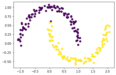
The spectral clustering works! There is one point that is misclassified but everything else is correctly classified.
Using Eigenvalues and Eigenvectors
The above method is relatively slow, and there is a faster shortcut using eigenvalues and eigenvectors. We find the eigenvalues of the inverse of D times (D minus A), and discover that the second smallest eigenvalue’s eigenvector contains the classes of the data.
# constructing matrix
L = np.linalg.inv(D)@(D - A)

# finding eigenvalues and eigenvectors
Lam, U = np.linalg.eig(L)

# sorting eigenvalues from smallest to largest
ix = Lam.argsort()

# removing smallest eigenvalue and its eigenvector
Lam, U = Lam[ix], U[:,ix]

# second smallest eignvector
z_eig = U[:,1]

plt.scatter(X[:,0], X[:,1], c = np.where((z_eig < 0), 0, 1))
We find that our spectral clustering algorithm works (and is a lot faster)! Now we synthesize our findings into one function, spectral_clustering, which takes in data and an epsilon value and outputs a true member cluster vector.
def spectral_clustering(X, epsilon):
"""
takes data and an epsilon value and outputs a true member cluster vector to correctly classify X into two clusters
"""
# pairwise distance matrix based on epsilon
A = (pairwise_distances(X) < epsilon).astype(int)
# fill diagonals with 0
np.fill_diagonal(A, 0)
# make an n x n matrix of zeros
D = np.zeros((n, n), int)
# fill diagonals with row-sum values
np.fill_diagonal(D, np.sum(A, axis = 1))
# create Laplacian matrix
L = np.linalg.inv(D)@(D - A)
# find eigenvalues and eigenvectors
Lam, U = np.linalg.eig(L)
# sort eigenvalues
ix = Lam.argsort()
# removing smallest eigenvalue and its eigenvector
Lam, U = Lam[ix], U[:,ix]
# second smallest eigenvector
z_eig = U[:,1]
# return true cluster membership vector based on signs of z_eig
return np.where((z_eig < 0), 0, 1)
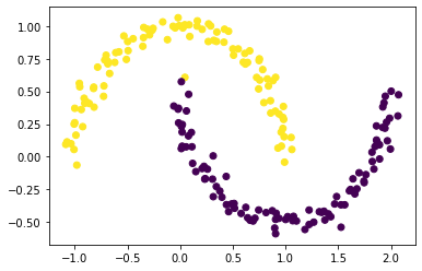
plt.scatter(X[:,0], X[:,1], c = spectral_clustering(X, epsilon))

Looks like the function works! There is one point on the top of the bottom moon that is incorrectly classified, however.
Experiments
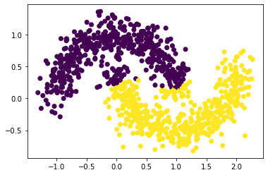
We run three experiments using a different make_moon dataset where the noise parameter is increased and the number of points is increased to 1000.
np.random.seed(1234)

# increasing the number of points to 1000
n = 1000

# make_moons where noise is increased to 0.1
X, y = datasets.make_moons(n_samples=n, shuffle=True, noise=0.1, random_state=None)
plt.scatter(X[:,0], X[:,1], c = spectral_clustering(X, epsilon))
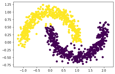
The clustering works relatively well; again, some top points from the bottom moon are misclassified.
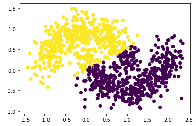
np.random.seed(1234)
n = 1000

# make_moons where noise is increased to 0.15
X, y = datasets.make_moons(n_samples=n, shuffle=True, noise=0.15, random_state=None)
plt.scatter(X[:,0], X[:,1], c = spectral_clustering(X, epsilon))
Here the clustering begins to fail a little, with more top points from the bottom moon and some bottom points from the top moon misclassified.
np.random.seed(1234)
n = 1000

# make_moons where noise is increased to 0.2
X, y = datasets.make_moons(n_samples=n, shuffle=True, noise=0.20, random_state=None)
plt.scatter(X[:,0], X[:,1], c = spectral_clustering(X, epsilon))
Looks like our spectral clustering algorithm doesn’t work as well—some of the points near the right end of the top moon and near the left end of the bottom moon are mixed. To be fair, however, a person would have difficulty separating the moons as well.
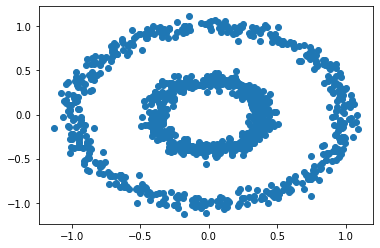
Bull’s Eye Data Set
We test our spectral clustering algorithm on the bull’s eye data set:
np.random.seed(1234)

# 1000 data points
n = 1000

# make two cocentric circles
X, y = datasets.make_circles(n_samples=n, shuffle=True, noise=0.05, random_state=None, factor = 0.4)
plt.scatter(X[:,0], X[:,1])
np.random.seed(1234)

# plot with spectral_clustering
epsilon = 0.4
plt.scatter(X[:,0], X[:,1], c = spectral_clustering(X, epsilon))
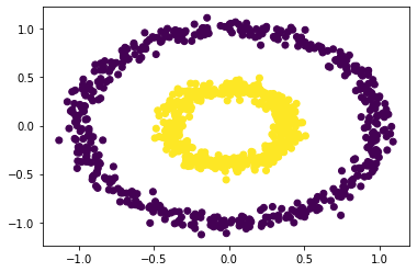
Looks like our spectral clustering algorithm works! Anytime we have a data set with “weirdly” shaped data, we can easily classify it.