Blog Post 5

In this post, we’re going to teach a convolutional neural network to distinguish between pictures of cats and dogs using the tensorflow library. We’ll use Datasets in tensorflow, and use data augmentation and transfer learning to improve our original model.

Load Packages and Obtain Data

To begin, we load packages and obtain our dataset. We load the following packages:

import os
from tensorflow.keras import utils, layers 
import tensorflow as tf
import matplotlib.pyplot as plt

To obtain our dataset, we use Google’s repository of dog and cat photos. We run the following code block to do so.

# location of data
_URL = 'https://storage.googleapis.com/mledu-datasets/cats_and_dogs_filtered.zip'

# download the data and extract it
path_to_zip = utils.get_file('cats_and_dogs.zip', origin=_URL, extract=True)

# construct paths
PATH = os.path.join(os.path.dirname(path_to_zip), 'cats_and_dogs_filtered')

train_dir = os.path.join(PATH, 'train')
validation_dir = os.path.join(PATH, 'validation')

# parameters for datasets
BATCH_SIZE = 32
IMG_SIZE = (160, 160)

# construct train and validation datasets 
train_dataset = utils.image_dataset_from_directory(train_dir,
                                                   shuffle=True,
                                                   batch_size=BATCH_SIZE,
                                                   image_size=IMG_SIZE)

validation_dataset = utils.image_dataset_from_directory(validation_dir,
                                                        shuffle=True,
                                                        batch_size=BATCH_SIZE,
                                                        image_size=IMG_SIZE)

# construct the test dataset by taking every 5th observation out of the validation dataset
val_batches = tf.data.experimental.cardinality(validation_dataset)
test_dataset = validation_dataset.take(val_batches // 5)
validation_dataset = validation_dataset.skip(val_batches // 5)

From here, we’ve created three Datasets: train_dataset, validation_dataset, and test_dataset. We also note that each image is 160 x 160 pixels.

We also run technical code to rapidly read our data.

AUTOTUNE = tf.data.AUTOTUNE

train_dataset = train_dataset.prefetch(buffer_size=AUTOTUNE)
validation_dataset = validation_dataset.prefetch(buffer_size=AUTOTUNE)
test_dataset = test_dataset.prefetch(buffer_size=AUTOTUNE)

Working with Datasets

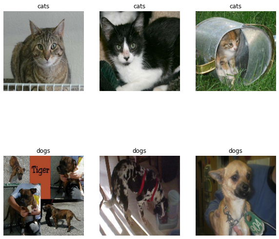
To visualize our dataset, we write a function that produces two rows of images: three images of cats in the first row and three images of dogs in the second row.

def two_row_visualization(train_dataset):

  # size of plot
  plt.figure(figsize=(10, 10))

  # for each image and label in one batch of 32 images
  for images, label in train_dataset.take(1):
    i = 0
    j = 0
    cats = 0
    dogs = 0

    # while the number of cat photos is less than three
    while cats < 3:

      # if ith image is a cat
      if label[i].numpy() == 0:

        # plot image as the cats + 1th image on the 2 x 3 grid
        ax = plt.subplot(2, 3, cats + 1)

        plt.imshow(images[i].numpy().astype("uint8"))

        # add cats label
        plt.title("cats")
        plt.axis("off")

        # plotted additional cat
        cats = cats + 1
      # move to next image
      i = i + 1

    # while the number of dog photos is less than three
    while dogs < 3:

      # if jth image is a dog
      if label[j].numpy() == 1:
        
        # plot image as the dogs + 4th image on the 2 x 3 grid
        ax = plt.subplot(2, 3, dogs + 4)
        
        plt.imshow(images[j].numpy().astype("uint8"))

        # add dogs label
        plt.title("dogs")

        plt.axis("off")

        # plotted additional dog
        dogs = dogs + 1
      # move to next image
      j = j + 1
    
two_row_visualization(train_dataset)

Check Label Frequencies

We create an iterator to help us see the number of images that are cats and the number of images that are dogs in the dataset.

labels_iterator= train_dataset.unbatch().map(lambda image, label: label).as_numpy_iterator()

count = 0

# for each image in train_dataset
for i in range(2000):

  # adds 1 if image is dog and 0 if image is cat
  count = count + labels_iterator.next()
print(count)

1000

Since our loop adds 0 if the image is of a cat and adds 1 if the image is of a dog, we see that there are 1000 images of cats in our dataset, which implies that there are 1000 images of dogs in our dataset.

The baseline machine learning model is the model that always guesses the most frequent label. Since our dataset is evenly split between cat and dog images, our baseline model would be 50% accurate. Any model that is better than 50% accuracy would be an improvement!

First Model

We use tf.keras.Sequential and a few tf.keras.layers to create our convolutional neural network. Below is our first model.

model1 = tf.keras.Sequential([

    # alteration of Conv2D and MaxPooling2D layers, with increase in number of filters for Conv2D layer and input_shape of 160 x 160 pixels and 3 values for RGB
    layers.Conv2D(32, (3, 3), activation = "relu", input_shape = (160, 160, 3)),

    layers.MaxPooling2D((2, 2)),
    layers.Conv2D(32, (3, 3), activation = "relu"),
    layers.MaxPooling2D((2, 2)),
    layers.Conv2D(64, (3, 3), activation = "relu"),
    layers.Flatten(),
    layers.Dropout(0.2),

    # final Dense layer of two classes (cats and dogs)
    layers.Dense(2)
])

# use adam optimizier and SparseCategoricalCrossentropy loss function, with accuracy as a metric
model1.compile(optimizer = "adam",
              loss = tf.keras.losses.SparseCategoricalCrossentropy(from_logits = True),
              metrics = ["accuracy"])

# train model on 20 epochs
history = model1.fit(train_dataset, 
                     epochs = 20, 
                     validation_data = validation_dataset)

# plot training accuracy over epochs
plt.plot(history.history["accuracy"], label = "training")

# plot validation accuracy over epochs
plt.plot(history.history["val_accuracy"], label = "validation")

# set labels
plt.gca().set(xlabel = "epoch", ylabel = "accuracy")

# show legend of training and validation
plt.legend()

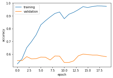
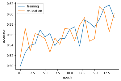
The accuracy of my model stabilized between 55% and 60% during training.

I did 5-10% better than the baseline.

In the visualization, training accuracy exceeds validation accuracy in later epochs. This indicates overfitting occurred.

Model with Data Augmentation

In our second model, we add some data augmentation layers to our model. Specifically, we introduce random flipping of images and random rotations of images to our model to help our model learn invariant features of our input images.

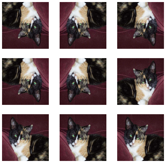
We demonstrate tf.keras.layers.RandomFlip() first.

data_augmentation = tf.keras.Sequential([
  # no parameters imply both horiziontal and vertical flipping
  tf.keras.layers.RandomFlip(),
])

for image, _ in train_dataset.take(1):

  # size of plot
  plt.figure(figsize = (10, 10))

  # first image is first in image array
  first_image = image[0]

  # show nine images
  for i in range(9):

    # plot image as the ith + 1 image on the 3 x 3 grid
    ax = plt.subplot(3, 3, i + 1)

    # apply random flip
    augmented_image = data_augmentation(tf.expand_dims(first_image, 0))
    plt.imshow(augmented_image[0] / 255)
    plt.axis('off')

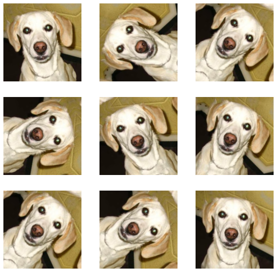
We then demonstrate tf.keras.layers.RandomRotation().

# parameter of 0.2 implies image will be rotated between 0.2 * 2pi radians clockwise and 0.2 * 2pi radians counterclockwise
data_augmentation = tf.keras.Sequential([
  tf.keras.layers.RandomRotation(0.2),
])

for image, _ in train_dataset.take(1):
  plt.figure(figsize = (10, 10))
  first_image = image[0]
  for i in range(9):
    ax = plt.subplot(3, 3, i + 1)
    augmented_image = data_augmentation(tf.expand_dims(first_image, 0))
    plt.imshow(augmented_image[0] / 255)
    plt.axis('off')

We then create our second model, this time with data augmentation.

# addition of RandomFlip() and RandomRotation(0.2)
model2 = tf.keras.Sequential([
    layers.RandomFlip(),
    layers.RandomRotation(0.2),
    layers.Conv2D(32, (3, 3), activation = "relu", input_shape = (160, 160, 3)),
    layers.MaxPooling2D((2, 2)),
    layers.Conv2D(32, (3, 3), activation = "relu"),
    layers.MaxPooling2D((2, 2)),
    layers.Conv2D(64, (3, 3), activation = "relu"),
    layers.Flatten(),
    layers.Dropout(0.2),
    layers.Dense(2)
])

model2.compile(optimizer = "adam",
              loss = tf.keras.losses.SparseCategoricalCrossentropy(from_logits = True),
              metrics = ["accuracy"])

history = model2.fit(train_dataset, 
                     epochs = 20, 
                     validation_data = validation_dataset)

plt.plot(history.history["accuracy"], label = "training")
plt.plot(history.history["val_accuracy"], label = "validation")
plt.gca().set(xlabel = "epoch", ylabel = "accuracy")
plt.legend()

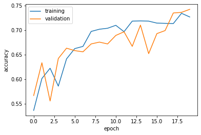
The accuracy of my model stabilized between 55% and 60% during training.

My validation accuracy for model2 is about the same as model1.

In the visualization, training accuracy and validation accuracy intertwine across epochs. This indicates no overfitting occurred.

Data Preprocessing

We then consider a simple transformation to the input data—in this case, a normalization of the RGB values of our input images. We create a preprocessing layer called preprocessor and add it into our model.

i = tf.keras.Input(shape=(160, 160, 3))
x = tf.keras.applications.mobilenet_v2.preprocess_input(i)
preprocessor = tf.keras.Model(inputs = [i], outputs = [x])

# addition of preprocessor layer
model3 = tf.keras.Sequential([
    preprocessor,
    layers.RandomFlip(),
    layers.RandomRotation(0.2),
    layers.Conv2D(32, (3, 3), activation = "relu", input_shape = (160, 160, 3)),
    layers.MaxPooling2D((2, 2)),
    layers.Conv2D(32, (3, 3), activation = "relu"),
    layers.MaxPooling2D((2, 2)),
    layers.Conv2D(64, (3, 3), activation = "relu"),
    layers.Flatten(),
    layers.Dropout(0.2),
    layers.Dense(2)
])

model3.compile(optimizer = "adam",
              loss = tf.keras.losses.SparseCategoricalCrossentropy(from_logits = True),
              metrics = ["accuracy"])

history = model3.fit(train_dataset, 
                     epochs = 20, 
                     validation_data = validation_dataset)

plt.plot(history.history["accuracy"], label = "training")
plt.plot(history.history["val_accuracy"], label = "validation")
plt.gca().set(xlabel = "epoch", ylabel = "accuracy")
plt.legend()

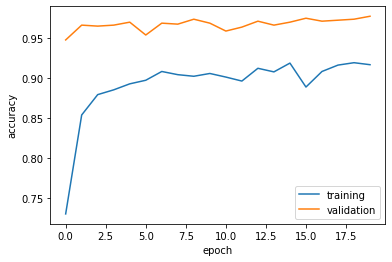
The accuracy of my model stabilized between 65% and 70% during training.

My validation accuracy for model3 is 10% better than model1.

In the visualization, training accuracy and validation accuracy intertwine across epochs. This indicates no overfitting occurred.

Transfer Learning

We finally use transfer learning, which uses a pre-existing base model and incorporates it into a full model. We use the MobileNetV2 model as a pre-existing base model in this case.

IMG_SHAPE = IMG_SIZE + (3,)
base_model = tf.keras.applications.MobileNetV2(input_shape=IMG_SHAPE,
                                               include_top=False,
                                               weights='imagenet')
base_model.trainable = False

i = tf.keras.Input(shape=IMG_SHAPE)
x = base_model(i, training = False)
base_model_layer = tf.keras.Model(inputs = [i], outputs = [x])

# usage of preprocessor, RandomFlip(), RandomRotation(0.2), base_model_layer, GlobalMaxPooling2D(), Dropout(0.2), and Dense(2)
model4 = tf.keras.Sequential([
    preprocessor,
    layers.RandomFlip(),
    layers.RandomRotation(0.2),
    base_model_layer,
    layers.GlobalMaxPooling2D(),
    layers.Dropout(0.2),
    layers.Dense(2)
])

model4.compile(optimizer = "adam",
              loss = tf.keras.losses.SparseCategoricalCrossentropy(from_logits = True),
              metrics = ["accuracy"])

history = model4.fit(train_dataset, 
                     epochs = 20, 
                     validation_data = validation_dataset)

plt.plot(history.history["accuracy"], label = "training")
plt.plot(history.history["val_accuracy"], label = "validation")
plt.gca().set(xlabel = "epoch", ylabel = "accuracy")
plt.legend()

The accuracy of my model stabilized between 95% and 100% during training.

My validation accuracy for model4 is between 40% better than model1.

In the visualization, training accuracy is below validation accuracy intertwine across epochs. This indicates no overfitting occurred.

Score on Test Data

We finally evaluate our final model on our test_dataset.

model4.evaluate(test_dataset)

6/6 [==============================] - 1s 67ms/step - loss: 0.0773 - accuracy: 0.9740 [0.07727044075727463, 0.9739583134651184]

We see that accuracy is 97%—a great success! We can accurately classify cat and dog images now.