Blog Post 6

In this post, we’re going to create a neural network that can distinguish between fake and real news, based on the title of the news article and its text using the tensorflow library. We also examine the embedding layer we use to visualize relationships between words in our dataset.

Acquire Training Data

We first import several libraries and download the dataset, which comprises of 22449 observations of news article titles and text, and a categorical variable, fake, indicating whether or not the article is fake (0 if the article is not fake, 1 if the article is fake).

import pandas as pd
from nltk.corpus import stopwords
import nltk 
nltk.download('stopwords')
import tensorflow as tf
from tensorflow.keras.layers.experimental.preprocessing import TextVectorization
import re
import string
from tensorflow import keras
from tensorflow.keras import layers
from tensorflow.keras import losses
import numpy as np

train_url = "https://github.com/PhilChodrow/PIC16b/blob/master/datasets/fake_news_train.csv?raw=true"
df = pd.read_csv(train_url)

Make a Dataset

We now write a function make_dataset() that creates a tensorflow Dataset without stopwords in title and text. After removing stopwords, the function outputs a Dataset with two inputs, title and text, and one output, fake.

def make_dataset(df):
    # English stopwords
    stop = stopwords.words("english")

    # remove stopwords from title
    df["title"] = df["title"].apply(lambda x: ' '.join([word for word in x.split() if word not in (stop)]))

    # remove stopwords from text
    df["text"] = df["text"].apply(lambda x: ' '.join([word for word in x.split() if word not in (stop)]))

    # create Dataset from modified title and text
    my_data_set = tf.data.Dataset.from_tensor_slices(
        (
            {
                "title" : df[["title"]], 
                "text" : df[["text"]]
            }, 
            {
                "fake" : df[["fake"]]
            }
        )
    )

    # set batch to 100 for faster runtime 
    my_data_set.batch(100)
    return my_data_set

data = make_dataset(df)

We also split off 20% of the dataset as validation data and 70% as training data.

# shuffle the data to ensure randomness
data = data.shuffle(buffer_size = len(data))

# size of training data
train_size = int(0.7*len(data))

# size of validation data
val_size = int(0.2*len(data))

# create training dataset
train = data.take(train_size)

# create validation dataset
val = data.skip(train_size).take(val_size)

# create testing dataset
test = data.skip(train_size + val_size)

# length of training data for base rate
len(train)

15714

We now calculate the base rate, the accuracy of our model if it keeps on making the same guess, which is the majority class.

# create an iterator
fake_iterator= train.unbatch().map(lambda x, fake: fake).as_numpy_iterator()
count = 0

# for each fake in train
for i in range(15714):

  # adds 1 if article is fake and 0 if article is real
  count = count + fake_iterator.next()["fake"]
print(count)

8223

Since there are 15714 observations in our training dataset, our base rate is 52.33%.

Create Models

We now create three different models, the first using only title as the input, the second using only text as the input, and the last using both title and text as the inputs.

We first create a text preprocessing layer to preprocess our text.

# size of our dataset vocabulary
size_vocabulary = 2000

def standardization(input_data):
    # set all letters to lowercase
    lowercase = tf.strings.lower(input_data)

    # remove punctuation
    no_punctuation = tf.strings.regex_replace(lowercase,
                                  '[%s]' % re.escape(string.punctuation),'')
    return no_punctuation 

vectorize_layer = TextVectorization(
    standardize = standardization,
    max_tokens = size_vocabulary,
    output_mode = 'int',

    # length of output vectors
    output_sequence_length = 500) 

vectorize_layer.adapt(train.map(lambda x, y: x["title"]))
vectorize_layer.adapt(train.map(lambda x, y: x["text"]))

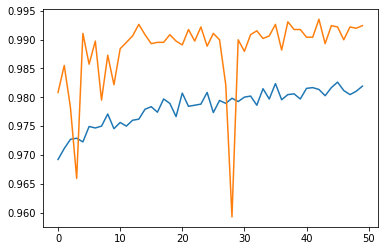
The first model only uses title.

title_input = keras.Input(
    # shape of title tensors
    shape = (1, ),

    name = "title",
    dtype = "string"
)

# vectorize title input
title_features = vectorize_layer(title_input)

# add an embedding layer to form relationships between words
title_features = layers.Embedding(size_vocabulary, 3, name = "embedding")(title_features)

title_features = layers.Dropout(0.2)(title_features)
title_features = layers.GlobalAveragePooling1D()(title_features)
title_features = layers.Dropout(0.2)(title_features)
title_features = layers.Dense(32, activation = "relu")(title_features)

# output has two classes
output = layers.Dense(2, name = "fake")(title_features)

# create model
model = keras.Model(
    inputs = title_input,
    outputs = output
)

# use adam optimizier and SparseCategoricalCrossentropy loss function, with accuracy as a metric
model.compile(optimizer = "adam",
              loss = losses.SparseCategoricalCrossentropy(from_logits=True),
              metrics=['accuracy']
)

# train on 50 epochs
history = model.fit(train, 
                    validation_data=val,
                    epochs = 50)

# plot training and validation accuracy across epochs
from matplotlib import pyplot as plt
plt.plot(history.history["accuracy"])
plt.plot(history.history["val_accuracy"])

/usr/local/lib/python3.7/dist-packages/keras/engine/functional.py:559: UserWarning:

Input dict contained keys [‘text’] which did not match any model input. They will be ignored by the model.

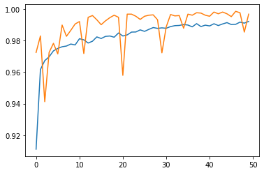
The second model only uses text.

text_input = keras.Input(
    # shape of text tensors
    shape = (1, ),

    name = "title",
    dtype = "string"
)

# vectorize text input
text_features = vectorize_layer(text_input)

# add an embedding layer to form relationships between words
text_features = layers.Embedding(size_vocabulary, 3, name = "embedding")(text_features)

text_features = layers.Dropout(0.2)(text_features)
text_features = layers.GlobalAveragePooling1D()(text_features)
text_features = layers.Dropout(0.2)(text_features)
text_features = layers.Dense(32, activation = "relu")(text_features)

# output has two classes
output = layers.Dense(2, name = "fake")(text_features)

# create model
model = keras.Model(
    inputs = text_input,
    outputs = output
)

# use adam optimizier and SparseCategoricalCrossentropy loss function, with accuracy as a metric
model.compile(optimizer = "adam",
              loss = losses.SparseCategoricalCrossentropy(from_logits=True),
              metrics=['accuracy']
)

# train on 50 epochs
history = model.fit(train, 
                    validation_data=val,
                    epochs = 50)

# plot training and validation accuracy across epochs
from matplotlib import pyplot as plt
plt.plot(history.history["accuracy"])
plt.plot(history.history["val_accuracy"])

The third model uses both title and text.

# vectorize title and text input
title_features = vectorize_layer(title_input)
text_features = vectorize_layer(text_input)

# shared embedding layer for both title and text
shared_embedding = layers.Embedding(size_vocabulary, 3, name = "embedding")
title_features = shared_embedding(title_features)
text_features = shared_embedding(text_features)

title_features = layers.Dropout(0.2)(title_features)
text_features = layers.Dropout(0.2)(text_features)
title_features = layers.GlobalAveragePooling1D()(title_features)
text_features = layers.GlobalAveragePooling1D()(text_features)
title_features = layers.Dropout(0.2)(title_features)
text_features = layers.Dropout(0.2)(text_features)
title_features = layers.Dense(32, activation='relu')(title_features)
text_features = layers.Dense(32, activation='relu')(text_features)

# concatenate title features and text features
main = layers.concatenate([title_features, text_features], axis = 1)
main = layers.Dense(32, activation='relu')(main)

# output has two classes
output = layers.Dense(2, name = "fake")(main)

# create model
model = keras.Model(
    inputs = [title_input, text_input],
    outputs = output
)

# use adam optimizier and SparseCategoricalCrossentropy loss function, with accuracy as a metric
model.compile(optimizer = "adam",
              loss = losses.SparseCategoricalCrossentropy(from_logits=True),
              metrics=['accuracy']
)

# train on 50 epochs
history = model.fit(train, 
                    validation_data=val,
                    epochs = 50)

# plot training and validation accuracy across epochs
from matplotlib import pyplot as plt
plt.plot(history.history["accuracy"])
plt.plot(history.history["val_accuracy"])

While all three models were successful, it seems as if our model that uses both title and text is most successful. Algorithms should use both title and text when seeking to detect fake news.

Model Evaluation

Now we test our best model on test data.

test_url = "https://github.com/PhilChodrow/PIC16b/blob/master/datasets/fake_news_test.csv?raw=true"
test_df = pd.read_csv(test_url)
test_data = make_dataset(test_df)

# evaluate third model on test dataset
model.evaluate(test_data)

22449/22449 [==============================] - 96s 4ms/step - loss: 0.0563 - accuracy: 0.9861 [0.05631158500909805, 0.9861018061637878]

Our model has 98.61% accuracy on the test data, so we didn’t overfit. We would detect fake news 98.61% of the time.

Embedding Visualization

Now we examine our embedding layer more. We create a visualization in plotly and examine words that are related to each other to see if they make sense.

# get weights from embedding layer
weights = model.get_layer('embedding').get_weights()[0]
vocab = vectorize_layer.get_vocabulary()

# use PCA with 2 components
from sklearn.decomposition import PCA
pca = PCA(n_components=2)
weights = pca.fit_transform(weights)

embedding_df = pd.DataFrame({
    'word' : vocab, 
    'x0'   : weights[:,0],
    'x1'   : weights[:,1]
})

import plotly.express as px 

# visualize words on a 2d graph
fig = px.scatter(embedding_df, 
                 x = "x0", 
                 y = "x1", 
                 size = list(np.ones(len(embedding_df))),
                 size_max = 2,
                 hover_name = "word")

fig.show()

We can see that insurance, sell, financial, living, and abortion are close to each other, near the center of our graph. This makes sense, since these topics could be related to women being able to afford abortions with insurance.